How much budget do I need with active learning?

TLDR: In this blog I discuss the expected budget of a experiment design (active learning campaign).

What is Active Learning?

Active learning (or design of experiment, if you got your education before the 2000s) is a machine learning (statistics) paradigm that helps to gather the most informative subset of a dataset to label (or measure) in order to improve the performance (whether raw or in terms of generalization, etc.) of your machine learning model.

Data is expensive, and accurate data is even more expensive, so usually, if you have some high-impact problem, the data is scarce and you need to plan your budget accordingly. For example, suppose you are working on protein design. You could create completely random mutants of your protein to understand the impact of mutations on its function, but maybe there’s a more efficient way to collect data. Maybe you want to cover a diverse set of sequences instead of sampling randomly from the pool. Maybe you want to minimize duplicates, or better yet, close duplicates in terms of function. Indeed, this is possible, and this is where active learning comes into play. A typical pipeline looks like the following:

1. Suppose your function $ f(x) $ has a certain complexity. This means the relationship between $ x$ and $ y$ is established. We do not know $ f $, but we know something about it. Examples include, but are not limited to (and possibly in combination):
   • $ f $ is linear
   • $f$ is a shallow 2-layer network
   • $ f $ is a Gaussian process (RKHS) with a certain kernel
   • $ f $ is positive, monotone, or convex, or has any other shape constraint
   • $ f $ is linear on the NN-embeddings $ \phi(x) $
   • $ f $ is a fine-tuned NN with a couple of gradient steps

2. The user measures $ y = f(x) + \epsilon$. Before experimenting, one has to establish the structure of the random noise $ \epsilon $—in other words, the error of measurement. Often, in practice, this is close to Gaussian for real-valued signals. For discrete signals, Poisson error might be more appropriate, but this is beyond the scope of this blog post.

3. Calculate a sampling strategy $ \pi $.

4. Sample or use a sampling strategy on the search space $ \mathcal{X} $. The search space is defined by the user.

5. Use part of the experimental budget and go back to step 1. Usually, you can update the estimate of your relationship, but the complexity remains. In other words, if you believe the neural network explains the relationship, you just update your belief about the parameters, not the actual relationship form.

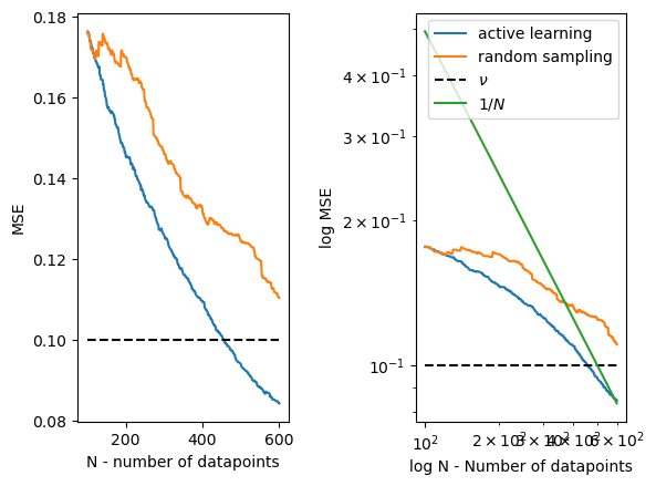
The promise of this scheme is that you would improve your performance much faster as a function of data compared to, say, randomized sampling. Such an example would look like the one below.

Even with random sampling, we reduce error, and we decrease it at the same asymptotic rate! With truly non-parametric models that allow us to change the norm of the function, the rate might differ from the typical $ 1/N $, but for any model with limited capacity, the only thing that changes is the constant. However, this constant can be very large and might even be unbounded for certain$ N_0 < N $! Hence, non-asymptotically, this can lead to significant improvements over other methods, such as random sampling, which might have a very large constant. The capacity is either the fact that the function has limited dimensions or, in functional spaces, that we assume the norm of the true non-parametric $ f $ is bounded in certain functional spaces. There is a very nice book by Grace Wahba [1] to learn more about non-parametric statistics.

Figure 1: MSE (mean squared error) of active learning vs. random sampling. Notice that eventually we approach the $ 1/N $ rate once the capacity of the model is reached.

How much data I need?

The above plot is post-hoc. We have collected the data and then evaluated the performance. If we want to achieve a fixed performance level, say at level $\nu$, how many datapoint do we need? We can read out this number from the graph above, see the dashed vertical line. However the graph is post-hoc execution, can’t always get this number before we start any of it, right? Well, it turns out this is the core thing what many theoretical works in active learning fields analyze.

Practically, there are couple of answers, but lets summarize them to effectively to two ways, one general, and one elegant. In both cases, we need to however understand how to construct instances of our problem; either by sampling or assume a regularity on our function.

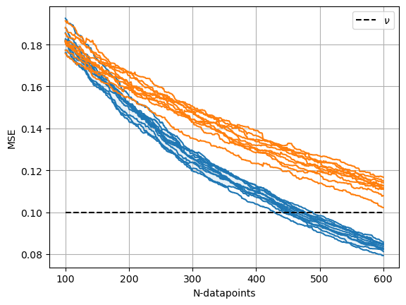
1. Simulations. We can always try to simulate the above with our guesses of possible $f$, and see what happens. See couple of simulations below, where each simulation is ran with a different $f$. The dashed lines are different instances of $f$. We end up with a budget given $\nu = 0.1$ at about 400-500 datapoints. We can perform similar analysis for random sampling as well.

1. Kernelized regression (RKHS or very related Gaussian processes) with Gaussian likelihood (or alike). For certain likelihoods and model classes, we can in fact calculate the worst-case expected error if we are in advance and in closed form (or even worst case maximum error in the dataset, though not covered here)!

In fact, it is so simple, let us derive it. I will derive it using the Hilbert space notation, where a kernel $k(x,y) = \braket{\phi(x), \phi(y)}$, and the function as $f(x) = \braket{f, \phi(x)}$. Since I am lazy I am just going to use a transposition as an indication for an inner product as $\braket{f, \phi(x)} = f^\top \phi(x)$.

The idea is simple, we observe corrupted values of $f(x) $ as $y = f(x) + \epsilon$, where $\epsilon$ has a known, in this case, Gaussian likelihood, and $f$ is the Hilbert space element.

In this specific derivation, we are going to calculate the average accuracy over the search space $\mathcal{X}$ as the performance metric we care about. The estimate we use to provide us the predictions and achieves this performance on this metric is the estimate $\hat{f}$ of $f$. The error is its deviation from the true $f$ on the whole search space:

The expectation is over the random noise realizations $\epsilon$. Let us use a shorthand for all the evaluated measurements as $X = [\phi(x_1), \dots \phi(x_n)]$, which gives a $\mathcal{H} \rightarrow \mathbb{R}^{n}$ operator, and adjoit $X^\top$. In the case of least squares regression, the estimator $\hat{f}$, can be represented as $\hat{f} = X^\top (K+\lambda I)^{-1}y = X^\top (K+\sigma^2 \lambda I)^{-1}(Xf + \epsilon)$. Plugging this estimating in, using the reproducing property and putting $f$ under the same bracket leads to:

Let us take the expectation with simple fixed parameters as $\mathbb{E}[\epsilon] = 0$, and $\mathbb{E}[\epsilon^2] = \sigma^2$, and $|f|\leq 1/\lambda$, bounded variation in Hilbert space. For proper generalization to arbitrary noise level consult the reference [2].

Let us define shortand for a covariance average span of the whole search space:

Effective Dimension - A metric that can hint.

After using all of this, we will arrive at:

\(E(X) \leq \sigma^2 \operatorname{Trace}\left(\left(\lambda I + \frac{X^\top X}{\sigma^2}\right)^{-1} V_s \right) ||f||^2\) Notice that this simple and elegant expression is able to bound the error. First or all notice that the operator $I$ and $X^\top X$ are $\mathcal{H} \rightarrow \mathcal{H}$ operators, hence we need to use matrix inversion lemma to evaluate them. Namely,

\(E(X) \leq \sum_{x}\frac{\sigma^2}{|\mathcal{X}|} \phi(x)^\top \left(\lambda I + \frac{X^\top X}{\sigma^2}\right)^{-1} \phi(x) = \frac{\sigma^2}{|\mathcal{X}|} \phi(\mathcal{X})^\top \phi(\mathcal{X}) - \phi(\mathcal{X}) X \left(\lambda I + \frac{X X^\top}{\sigma^2}\right)^{-1}X\phi(\mathcal{X}),\) where $\Phi(\mathcal{X})$ is the stacked embeddings of the whole search space. This can be conveniently evaluated in the computer by using the fact that $\Phi(x)\Phi(\mathcal{X}) = k(x,x_s)$ where the vector is of size $\mathcal{X}$ on the index $s$.

Now comming to the center of the derivation. We can in fact ask what is the lowest possible value of $E$, given the fixed budget $n$, how much can I optimize this? In paricular,

This is a challenging discrete optimization problem. Its in fact known to be NP-hard in its simplest variant [3]. However, upon performing a probability relaxation, where inclusion of $x \in \mathcal{X}$ changes to probability whether $x$ is $\eta(x)$, we can reformulate the problem as:

This is a convex optimization problem that can be easily solved using interior point methods, mirror descent or frank-wolfe. This quantity is often referred to as effective dimension of the problem.

Notice clearly that this number increases with the $\sigma^2$ but also decreases with $\lambda$. The more regularized the problem the less complexity and the more noice the less possible recovery.

As a sidenote, in the statistical literature the above quantity appears in generalization bounds most commonly. In fact it arises when evaluating the value of $E$ when sampling iid data evaluated on the same iid distribution in expectation (generalization). This quantity hence mostly features in works that characterize complexity of generalization of non-parametric models in machine learning.

Pratical Note and Example

In terms of overall numbers, this number is not representing anything much practically relevant since we need either the regularization value (and hence bound on the $f$; or bound on the $||f||$ which will imply regularization). Despite not knowing $\lambda$ precisely it allows us to do is to understand relative budgetary constraints. Namely, if I am at accuracy $\nu$, I need $n(\nu)$ data in order to make sure $\min_n \min_\eta E_n(\eta)-\nu < 0 $, the extra experimental effort to increase the accuracy to $2\nu$ is $n(2\nu)$, and these numbers are however informative. If I want to increase the accuracy by twice, we can see how many more datapoint we need.

Let us take a practical example, we have a trained neural network embeddings from a foundational model in this case support ESM2 [4]. A versatile model for protein embeddings based on sequence information. In goes sequence $x$, and out comes embedding $\phi(x)$ a fixed length vector.

Now we will use this to define a kernel as $k(x,y) = \exp(-\sum_i\gamma_i(\phi_i(x)-\phi_i(y))^2)$.

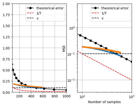
We will use a dataset from our work [5] designing a novel Metallo-enzyme. This dataset contains 3k+ sequences. We want to understand how much the average error improves as we increase the sample size by follwoing optimal active learning sampling strategy. See the worst-case calculation $E$ as theoretical error:

Figure: Expected worst-case (for the worst function) mean squared error on a search space of streptavidin variants.

If we look at these plots of the above quantity along with the simulations, we see the worst case performance is not far away from the simulated one.

Code

To calculate theoretical capacity of your model and/or embeddings can be reconstructured using my library stpy and doexpy with little effort as you can see bellow. These packages can be found on my github.

from stpy.continuous_processes.nystrom_fea import NystromFeatures
from stpy.kernels import KernelFunction
from stpy.helpers.helper import interval_torch
from mdpexplore.env.bandits import Bandits
from mdpexplore.functionals.doe_static_functionals import DesignA
from mdpexplore.convex_solvers.frank_wolfe import FrankWolfe
from mdpexplore.feedback.feedback_base import EmptyFeedback
from mdpexplore.solvers.dp import DP
from mdpexplore.policies.summary_policies.density_policy import DensityPolicy
from mdpexplore.mdpexplore import MdpExplore
import torch 
import matplotlib.pyplot as plt

# list of kernels
kernels = [KernelFunction(kernel_name="squared_exponential", gamma=0.1), 
           KernelFunction(kernel_name="squared_exponential", gamma=0.5)]
# names of the kernels
names =["RBF $\gamma = 0.01$", "RBF $\gamma = 0.1$", "RBF $\gamma = 0.5$"]

# define the discretized inveral [-1,1]
x = interval_torch(128,d = 1)*2

# We calculate finite dimensional embeddings for the intervals for easier calculation
# We use Nystrom features with thresholdon explained variance
embeddings = []
for k in kernels:
    Nystrom = NystromFeatures(k, m = None, approx = 'svd-explained')
    Nystrom.fit_gp(x, None, explained_variance = 0.999)
    embeddings.append(Nystrom.embed)

# define the budget of the experiment 
Ts = torch.logspace(1,10,10,base=2)
sigma = 0.05
for name, emb in zip(names,embeddings):
    values = []
    
    for T in Ts: 
        phi = emb(x)
        
        # define the environment
        env = Bandits(
            action_space=phi
        )
        
        # define the problem
        design = DesignA(
            env=env,
            lambd=1.,
            dim = 1,
            V = phi.T@phi/(sigma**2))
        
        # define the convex solver
        convex_solver = FrankWolfe(env,
                                   objective=design,
                                   num_components=10*phi.size()[1],
                                   solver=DP,
                                   step="line-search",
                                   SummarizedPolicyType=DensityPolicy,
                                   accuracy=1e-5)
        
        # define the feedback class
        feedback = EmptyFeedback(env, design)
               
        # Bandit environment 
        env = Bandits(action_space=phi)
        
        me = MdpExplore(
            env=env,
            objective=design,
            convex_solver=convex_solver,
            verbosity=0,
            feedback=feedback,
            general_policy='markovian')
        
        val, opt_val = me.run(
            episodes=int(T))
        
        values.append(-sigma**2*opt_val/T)
    plt.loglog(Ts, values,'o-', label = name)
#plt.loglog(Ts,1/Ts,'k--')
plt.xlabel("Number of Experiments")
plt.ylabel("Achievable Accuracy")
plt.legend()

References

1. Grace Wahba, Spline Models for Observational Data, 1990, CBMS-NSF Regional Conference Series in Applied Mathematics.
2. Experimental Design for Linear Functionals in Reproducing Kernel Hilbert Spaces, NeurIPS 2022
3. Cerny, Hladik Two complexity results on c-optimality in experimental design, 2012, Computational Optimization and Applications 51(3):1397-1408
4. Lin et. al., Language models of protein sequences at the scale of evolution enable accurate structure prediction, bioRxiv https://www.biorxiv.org/content/10.1101/2022.07.20.500902v1
5. Vornholt, T., Mutný, M., Schmidt, G. W., Schellhaas, C., Tachibana, R., Panke, S., Ward, T. R., Krause, A., & Jeschek, M. (2024). Enhanced sequence-activity mapping and evolution of artificial metalloenzymes by active learning. ACS Central Science. https://doi.org/10.1021/acscentsci.4c00456
6. Mojmir Mutny, Modern Adaptive Experiment Design: Machine Learning Perspective, 2024. PhD Thesis ETH Zurich.*